The Structural Chemistry of Lanthanide Compounds

This is an excerpt from the initial draft of Chapter 6 of <Structural Chemistry>, with specialized original content, illustrating, from authors (FC) pioneering breakthroughs, what is special with calculations on lanthanides.
At the end of the text, practical illustration of the discussed example is given.
6.6. The specifics and subtleties of electronic structure of lanthanide complexes.
6.6.1. The puzzle of the f orbitals in molecule
There is a relative scarcity of ab initio reports on lanthanide complexes, because of hidden technical difficulties, related with facts that can be pointed as the case of the weakly interacting f electrons and the non-aufbau nature of the f shell (Ferbinteanu et al 2015). Namely, the maximum of the r2R4f(r) profile for the 4f orbitals, is at about 0.4-0.5 A, while the ionic radius of trivalent lanthanides goes around 1 A. This determines a low propensity of the electrons placed in the f shell to interact with the surroundings (ligands, lattice|). In the sense of orbital theories, this implies occupied molecular orbitals with predominant, almost pure, f-type AO nature. Being closer to the nucleus and shielded from outer effects, the f electrons experience rather high absolute values of negative orbital energies, a situation that can end with f-based MOs placed lower that other occupied orbitals of the assembly. Except the trivial cases of lanthanide systems with no f electrons (like the complexes of trivalent lanthanum, La3+, with f0 configuration) or closed shell complexes (like those of lutetium, Lu3+, with f14 configuration), this would imply schemes with unpaired electrons placed bellow other levels, like doubly occupied ligand-based orbitals, or other singly occupied d-type orbitals from transition metal sites (in hetero-metallic complexes), namely non-aufbau occupations. The finding of an actual non-aufbau pattern may depend on the canonicalization technique of the used method, being in this way prone to some conventions on the defined mean field of electrons, but intuitively is reasonable to conceive the situation of weak interaction as described by a drastic separation in the MO energy diagram.
The lanthanide electronic structure is the ground for the interplay of Ligand Field (LF) and Spin Orbit (SO) effects, determining the effect of magnetic anisotropy, the lanthanide complexes (Cotton 2006; Benelli and Gatteschi 2002; Tanase and Reedijk 2006), having, for this reason, a special place in the tableau of molecular magnetism. The intrinsic anisotropy of the f ions is the key ingredient needed to achieve systems behaving as magnets at molecular scale, leading to Single Molecule Magnets, (SMMs) (Sessoli and Powell 2009; Mishra et al 2004) and even Single Ion Magnets (SIMs), the chosen system being a prototypic case for this last type of behavior.
The SMMs and SIMs are known also for transition metal ion compounds. The SMM can be thought as the analogue of a magnetization domain, known from solid state magnetism, isolated at molecular level. The investigation of SMMs represents the way for the consistent deeper insight in the quantum nature of the magnetism, the systems being also possible future materials for the magnetism at nanoscale, in the applied sciences. In this context, the SIMs are most interesting, bringing the level of miniaturization, down to a single momentum per molecule. Another interesting class is those of so-called Single Chain Magnets (SCMs) (Costes et al 2004, Ferbinteanu et al 2005), contouring the idea of one-dimensional magnets.
6.6.2. An intermezzo on the magnetic anisotropy
Since the magnetic anisotropy is an important issue in the fundamental and applied science of molecular properties, (Cimpoesu and Ferbinteanu 2014) basically the dominating paradigm of the new generation of problems in the molecular magnetism of the last decade, and the lanthanide complexes are regarded as some of the interesting objects in this field, it is worth presenting the topic in few words.
The nature of magnetic anisotropy, illustrated in the Figure 6.26, can be resumed as follows: although the spin of the electron can be regarded as the smallest quantum magnet, it cannot determine by itself a system to behave as magnet, at molecular and then, at macroscopic scale. To make a magnet, a fixed North-South pole axis must be ensured, with respect of the 3D frame where the system exists. However, the spin of the electron and its attached magnetic moments comes somehow out of our 3D space, from relativistic behaviour, as described in Chapter 1. Therefore, the spin magnetic moment is projected isotopically in a Cartesian axis of the molecule or of the solid lattice. In turn, the other source of magnetism, the orbital momentum, is the manifestation that can produce directed 3D magnetic moments. Roughly speaking, the orbital momentum can be regarded as a microscopic analogue of a current in a coil, since concerns the movement of the electron in the space. The orbital degeneracy, enabling the change of density, without energy cost, is the necessary factor. Because of spherical symmetry, the orbital, or combined spin-orbital momentum of the free atoms and ions, is also isotropic, but the symmetry of local environments determines, via Ligand Field factors, the anisotropy of magnetic properties of a given site.
The low involvement of the f shell in the bonding, namely the low Ligand Field splitting conserves a quasi-degeneracy, reaching a compromise between the partial survival of orbital component of the magnetism and the appearance of anisotropic features.
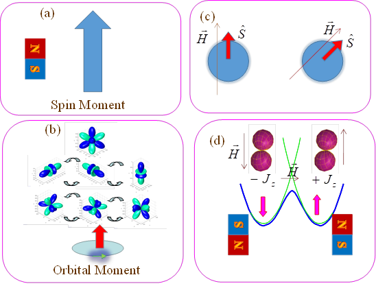
Fig. 6.26. Synopsis of the ingredients of the magnetic anisotropy at the level of ion-in-molecule: (a) the spin magnetic moment of the electron is the "smallest permanent magnet" ; (b) the orbital magnetism, related to the free movement of electrons between equivalent (degenerate) orbitals is, figuratively, the equivalent of the magnetic field induced by a coil of current; (c) the pure spin is isotropic- the magnetization follows freely the field and the magnetization tensor is a sphere (d) the magnetic anisotropy (non-spherical, e.g. bi-lobe magnetization map) and the energy barrier between opposed spin projections states are the sine qua non premises of building systems behaving as magnets.
At the end, the spin-orbit coupling, determines also the spin component of magnetic moment to behave anisotropically, the most frequent pattern being the formation of the so-called easy axis, along which the magnetic moment is aligned. The quasi-degenerate orbital terms and a large spin-orbit coupling are making the f-elements most interesting ingredients for magnetic materials. The d-type transition elements, having higher ligand fields contain the orbital magnetic components only in small traces, treatable in the limits of perturbation theory, having consequently lesser anisotropic propensities.
For a final touch must note one more parameter in the list of causal factors that are making a molecular system to act as a magnet. Thus, having an established easy magnetization axis is not yet enough, since two opposite directions of the magnetic moment can be accommodated, at the same energy- in the absence of a magnetic field. However, this means that we can have a rapid, uncontrolled, flipping of the North and South poles. To repair this indeterminate situation, fixing a given stability of poles, must have an energy barrier between equivalent magnetic polarizations. Whether the formation of the easy axis is a rather local phenomenon, caused by electronic structure of the metal ion and the Ligand Field parameters of the immediate environment, the reaction coordinate of a barrier between opposed magnetizations is a more complicate molecular deal, not yet completely treatable in clear a structural methodology. The so-called relaxation coordinate is a combination of soft molecular vibrations and lattice modes. The supra-molecular extension of the relaxation coordinate determines the next causal subtlety, namely the cooperativity that makes a molecular structure to behave as magnet at larger scale, nano-, meso- or macro. Although there are yet few steps to be taken in the complete property engineering of magnetic materials, by the leverage of causal structure-property relationships, the first steps can be trustfully taken, with the help of available conquests in molecular structure and ancillary tools of phenomenological models, such as the Ligand Field effective Hamiltonian.
6.6.3. The non-aufbau nature of the f-shell in the molecular orbital pictures
The lanthanide complexes form series whose congeners are closely similar each to other (Cotton and Wilkinson 1988), with respect of molecular geometries, synthetic procedures and general chemical behavior. The cause resides in the inner character of the f shell both in the energy scale and also as atomic radius. Therefore, the configuration of the fn shell does not affect the chemical bonding, while it determines the magnetic and optical properties. Then, although, in geometrical respects, the lanthanides are similar, the electronic structure and optical or magnetic consequences vary drastically among congeners.
As illustration of the specifics of f-type complexes, the case of the bis-(phtalo-cyaninato) terbium complex, [Pc2TbIII]-, is taken, (Ishikawa et al 2005; Ishikawa et al 2003) the system having the advent of a relative simplicity. For more simplification, on the ground of mutual comparability of lanthanide complexes, the illustration of the non-aufbau issue is obtained considering the [Pc2Lu]- complex as representative for the whole [Pc2Ln]- series, made with Ln3+ ions carrying unpaired electrons and magnetic moment. The Lu(III) congener, having closed f shell, does not imply itself a non-aufbau case. However, by contiguity, one may assume that at least analogues from the end of the lanthanide series (i.e. going backwards, the Yb3+, Tm3+, Er3+ ions) share the same pattern of orbital diagram. Considering the data displayed in Figure 6.27 and Table 6.11 on the [Pc2Lu]- complex, one may think, indeed, that when the f shell becomes incompletely filled, namely, it is found in a non-aufbau situation. One observes that the f -type orbitals are deeply placed in the energy scale, having more than one hundred ligand-type doubly occupied MOs above.
The [Pc2Lu]- was treated with B3LYP functional, using SBKJC (Day et al 1996; Jensen 2001) effective core potential (ECP) and basis set for Lu, 6-311G* basis set for the N atoms and 6-31G for the C and H ones. The Table 6.11 has two sections: the left one contains the MO sequence where the f-like components are placed, from 152 to 159 order indices, the identification being made by population analysis, and also by drawing the molecular contours, shown in Figure 6.28, along with the graphical representation of the MO energies. The right part of the Table 6.11 contains the frontier sequence, with the HOMO placed in the 277-th position.
In the [Pc2Lu]- complex, one observes also an accidental mixing between f-type and the ligand orbitals. Thus the MOs 152 and 153 (corresponding to e3 degenerate couple in the D4d symmetry), have only about 85% f content. The f-type with b2 symmetry is smeared among the MOs 154 (45%) and 159 (55%).
Table 6.11. The MO sequences containing the MOs similar to f AOs (left table) and the frontier MO part (right table) of the [Pc2Lu]- complex. The entries contain the order indices, MO energies (in eV), the occupation numbers of the MOs and the Mulliken population of the Lu atom in each MO.
|
# MO |
e (eV) |
Occ. |
Pop. (Lu) |
# MO |
e (eV) |
Occ. |
Pop.(Lu) |
|
151 |
-12.626 |
2 |
0.00 |
271 |
-4.112 |
2 |
0.001 |
|
152 |
-12.607 |
2 |
1.68 |
272 |
-4.073 |
2 |
0.000 |
|
153 |
-12.607 |
2 |
1.68 |
273 |
-4.071 |
2 |
0.000 |
|
154 |
-12.599 |
2 |
0.89 |
274 |
-3.916 |
2 |
0.019 |
|
155 |
-12.560 |
2 |
1.92 |
275 |
-3.804 |
2 |
0.012 |
|
156 |
-12.560 |
2 |
1.92 |
276 |
-2.678 |
2 |
0.000 |
|
157 |
-12.544 |
2 |
1.94 |
277 |
-2.000 |
2 |
0.000 |
|
158 |
-12.544 |
2 |
1.94 |
278 |
-0.229 |
0 |
0.000 |
|
159 |
-12.501 |
2 |
1.10 |
279 |
-0.229 |
0 |
0.000 |
|
160 |
-12.408 |
2 |
0.15 |
280 |
0.090 |
0 |
0.000 |
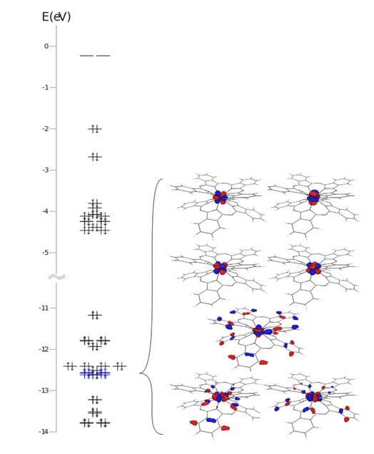
Fig. 6.27. The MO diagram of the [Pc2Lu]- complex illustrating the inner shell nature of the f-type MOs, that determines the non-aufbau situation of the [Pc2Ln]- systems with incomplete f shell.
The hybridization between f shell and ligand MOs is not expected, from physical point of view, its occurrence being a drawback of single-determinant methods in the account of the parts in weak interaction. In other words, there may be distant orbitals having comparable energies, which do not enter in interaction and mixing, but the DFT frame may not properly discriminate this physical separation.
For the proper account of f-type complexes must go to the multi-configuration calculations that will cure the spurious mixing, by their intrinsic capacity in representing the weakly interacting sub-systems. Besides, the multi-configuration is the correct representation of a quasi-degenerate situation, as is expected here, in the case of complexes of lanthanides with degenerate groundstates, as free ions, and quasi-degenerate in molecules. In degenerate circumstances are all the open-shell f-ions, except the sole situation of f7 configuration, reached by Gd3+ or Eu2+ systems (that show orbitally non-degenerate 8S ground term). Because of weak interaction with the environment, the split of the ground orbital multiplets is expected to be small, as is also known from the rather long practice with phenomenological Ligand Field models on the spectroscopy and magnetism of the lanthanide compounds. Typically, the whole gap of the LF split on f-type orbitals, or on the spectral terms (disregarding, formally, the spin-orbit effects) is about several hundreds of reciprocal centimeters (Newman 2000). Then, in the general case of low symmetry, is expected that any component of a molecular spectral term should be expressed as combination of Slater determinants known to give a valid description of the free ion, facing then the need for a multi-configuration method. Of course, the most immediate technical answer, if a computation is aimed, is the CASSCF (Complete Active Space Self Consistent Field).
The chosen case study is the [Pc2Tb]- phtalocyaninate-terbium(III) complex (Ishikawa et al 2005; Ishikawa et al 2003). The bis(phtalocyaninato) lanthanide systems show spectacular properties, such as the Single Ion Magnet (SIM) behavior for the [Pc2Tb]-, [Pc2Dy]- or [Pc2Ho]- congeners (Ishikawa et al 2005b; Ishikawa et al 2005c; Ishikawa 2010), or interesting manifestations of the redox modified, surface deposited, molecules (Branzoli et al 2009; Katoh et al 2009; Stepanow et al 2010). The [Pc2Tb]- system is well suited for the proposed theoretical tests: i) the molecule can be idealized to the D4d symmetry, where the LF parameter set becomes simple; ii) Ishikawa performed a remarkable Ligand Field (LF) analysis by fit to experimental magnetic data (Ishikawa et al 2003; Ishikawa et al 2002), having then a valuable comparison frame; iii) the post-calculation analysis is particularly simple for the f8 configuration, since the split of the states originating from the 7F spectral term can be equated in terms of LF nominal parameters only, without explicit two-electron part.
Usually, the CASSCF calculation needs a carefully chosen orbital set, to be sure that the active space (the sequence of orbitals where all the excitations of a defined number of electrons are developed) represents well the desired physical meaning. In our case, the active space will consist in the MOs resembling the f-type AOs in the molecule. In normal situation, a cheap single-determinant method, Hartree-Fock or DFT, can be used as preamble, their output MOs entering as input guess for the subsequent CASSCF. The above discussion about the fact that f-type orbitals may be hidden among other orbitals, which are not of interest for the active space construction, puts in conceptual and technical difficulty the launch of a CASSCF procedure. If for instance, if try a restricted open shell Hartree-Fock on a f complex, attempting to find in this way the f-type MOs, severe convergence problems are faced, because, used in routine mode, the program will aim for an impossible aufbau solution. Certain codes, like ADF, allow the control of orbital population and the imposing of a non-aufbau configuration. However, for large molecules will be difficult to figure in advance the orbital window in which the f-type MOs are expected. We assign to this kind of situation the lack of ab initio type accounts of molecular lanthanide complexes. Probably, many peoples tried, unaware about the specifics of lanthanide systems, failing to get a good orbital guess by HF or DFT preliminaries, refraining subsequently to report the negative results. The situation was in sharp contrast with the account of transition metal ion systems, whose spectroscopic and magnetic properties are already since several decades well complemented by the electronic structure calculations (Kahn 1993). The lanthanides, although formed a good part of the experimental molecular magnetism, particularly in the conjuncture with the magnetic anisotropy paradigm were not, until relatively recently, treated proportionate with their importance.
Must point that in the solid-state DFT, namely in the band structure calculations by plane waves and related methods, the lanthanide lattices can be tackled, especially making use of DFT+U methods, that alleviate a part of the problems induced by the f shell. However, as matter of principle, the DFT still faces limitations in the possibility to account orbital multiplicity and the quasi-degenerate situations. At the same time, the worlds of molecular and solid state DFT are somewhat disconnected and, in spite of the fact that the plane-wave methods can be applied to molecules too (encasing them in large boxes, treating a periodic collection of almost non-interacting identical entities), there are not many applications of this sort in the mainstream molecular magnetism, the chemists having a certain refrain in adopting here the physicists language.
The authors of the present book claim pioneering breakthroughs in the ab initio account of real scale lanthanide complexes, pointing the existing conceptual problems and presenting ways to circumvent the technical difficulties. A first work was dedicated to a gadolinium complex (Paulovic et al 2004) (namely a system with non-degenerate orbital groundstate) following analyses dealing with systems presenting the issues of orbital multiplets and the spin-orbit coupling (manifesting therefore magnetic anisotropy) (Ferbinteanu et al 2006; Cimpoesu et al 2012). Ulterior to our methodological resolutions, other ab initio works appeared, (Chibotaru 2013), but the first principle treatment of lanthanide complexes still remains a rather rare and delicate issue.
Our solution to the problem of starting active space was simple: the procedure was initiated with orbitals merged from the wavefunctions resulted from a preliminary account on the free lanthanide ions and SCF on remainder of the system (ligands or d-type complexes). For the ligands, HF or DFT methods can be used, without facing problems, while for the free lanthanide ions the CASSCF can be employed in good conditions, since here there is no non-aufbau issue or accidental degeneracy with other orbitals. The merging is realized by the help of an auxiliary code, putting on the diagonal blocks of the LCAO matrix and zero components between the elements of the constituting fragments.
There also alternatives to the previously drawn way. One, based on the presumed relative similarity of the lanthanide series, would be based on the orbitals of a closed shell calculation of the lutetium analogue, picking the orbitals with the most f character. Besides, a localization step can be considered, to filter the desired f-AO alike purity, reordering properly the result of procedure, so that can be taken as the orbitals of the active space. In principle, the identified f-components of lutetium can be taken as starting point for multi-configurational calculation of other lanthanide systems.
Another way can be based on unrestricted HF or DFT calculations. The unrestricted single determinant approaches of the paramagnetic lanthanide complexes are yet possible and usually convergent in good conditions, in spite of disputable meaning of the solution (the inquiries about the picking of a good single component from a quasi-degenerate bunch of interacting states). However, if consider the gadolinium complexes, having a single configuration, with seven parallel electrons in the seven f orbitals, the unrestricted solution can be physically meaningful. It will look also in a non-aufbau style, in spite of the fact that for the unrestricted frame, where α and β orbitals are independent of each other.
However, the seven f-type α electrons in a large complex will be found buried deep in the energy diagram, below many ligand-based orbitals. Calling, after the unrestricted step, for the obtaining of the so-called unrestricted natural orbitals (UNOs), one retrieves a set resembling a restricted open-open shell result, with a set of orbitals close to the double occupations, a series of almost singly occupied MOs and others with low occupation, originating from nearby the frontier, aside the many functions with definite virtual nature (the UNOs result with fractional populations). Therefore, the UNOs with occupations close to unity, resulted after the unrestricted HF or DFT on a gadolinium analogue, can be taken as start for other lanthanide congeners, provide that the basis sets have the same structure along the f series (as usually is the case). Being placed at the middle of the lanthanide series, the UNO-based gadolinium congener can be a good calculation starter for any congener complex.
The quasi-degeneracy of the lanthanide complexes is an occasion for the illustration of the state-averaged version of the CASSCF. Namely, designing the orbitals as resulting from density matrices mediated over a set of states, representing the degeneracy of the atomic spectral term of the given lanthanide ion, on reaches a better balance in the account of the f shell in the molecule, as it undergoes only small perturbation. If optimize separately each state, one may obtain overestimations, due to uncontrolled mutual departures of orbitals resulted from the different self-consistent processes.
The calculations of the [Pc2Tb]- unit, performed with the GAMESS code (Schmidt et al 1993), consisted in state averaged CASSCF(8,7) procedure, related with the eight electrons in the seven orbitals, corresponding to the f8 configuration of the Tb(III) ion. The SBKJC effective core potential and basis set was chosen for lanthanide atom, 6-311G* for the nitrogen atoms and 6-31G for the C and H skeleton. The averaging was taken on the seven states, representing the degeneracy of the F ground term of this configuration (more exactly 7F, if consider the spin index, or 7F6, if consider the spin-orbit coupling, ignored for the beginning).
The extension of active space to include 5d and 6s AOs on Tb(III) has little effect. The spectral terms resulted from the split of the 7F term of Tb(III) in the D4d point group are 7A1, 7E1, 7E2, 7E3. These can be simply characterized as the placement of the b electron of the f8 configurations into the b2, e3, e2, e1 respective sequence of f AOs. Here we use the convention of labelling the spectral terms by capital letters, while those dedicated to the orbitals are non-capitalized. The relationship between the D4d symmetry labels of f AOs vs. those of the spectral terms originating from the 7F atomic one, can be understood as follows.
The orbital symmetry of the half-filled shell f7 is B2, so that the labels of spectral terms resulted from the f8 configuration can be presented as product of a B2 background with those of running orbital components: e.g. 7A1=B2xb2 when the b electron is placed in the b2 -type f orbital, 7E1=B2xe3 , when it is accommodated in the e3 set, etc. The b2, e3, e2, e1 labels can be put in direct connection with the m=0, +/-1, +/-2, +/-3 quantum numbers, or with the s, p, d and j symbols of axial symmetry. The quantization is made with respect of the fourfold axis of the [Pc2Tb]- complex. With respect of the spectral terms, the m=0, +/-1, +/-2, +/-3 indices and the respective the e0, e1, e2, e3 energies can be assigned to the 7A1, 7E1, 7E2, 7E3 series. Because all the components of the 7F term have the same two-electron content, the ei, (i= 0..3) spectral energies can be taken as the LF scheme itself.
Table 6.12. Computed absolute and relative CASSCF energies and assignment with respect of LF scheme and the splitting of the 7F term of Tb(III).
|
Term |
LF |
Computed CASSCF states (Hartree) |
Relative energy with respect of groundstate (cm-1) |
Energy with respect of the barycenter (cm-1) |
|
|
7E1 |
e3 |
-3439.7284660040 |
0.0 |
-426.6 |
|
|
|
|
-3439.7284660040 |
0.0 |
-426.6 |
|
|
7E3 |
e1 |
-3439.7263867480 |
456.3 |
29.8 |
|
|
|
|
-3439.7263867480 |
456.3 |
29.8 |
|
|
7A1 |
e0 |
-3439.7259720510 |
547.4 |
120.8 |
|
|
7E2 |
e2 |
-3439.7249895980 |
763.0 |
336.4 |
|
|
|
|
-3439.7249895830 |
763.0 |
336.4 |
|
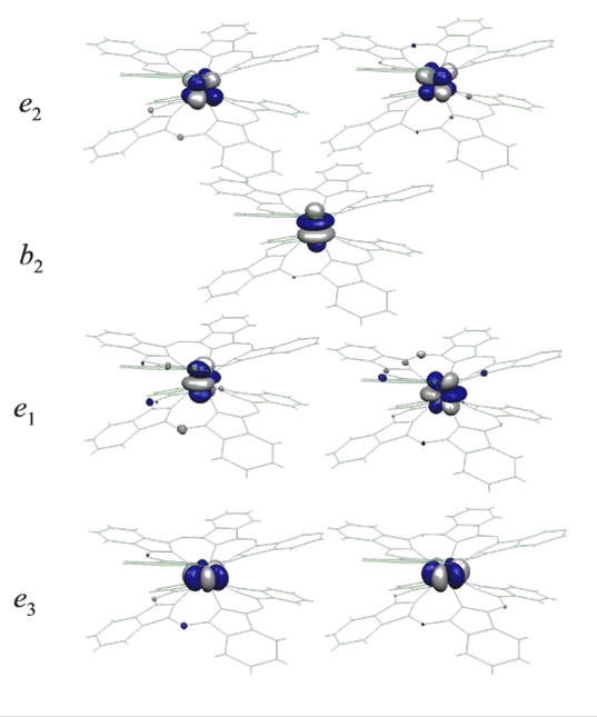
Fig. 6.28. The canonical MOs optimized from state-averaged CASSCF(8,7) calculation on the [Pc2Tb]- complex unit. Note the pure f character of the MOs.
The CASSCF calculation on [Pc2Tb]- anion yielded the 7E1 < 7E3 < 7A1 < 7E2 order correlated with to the placement of the b electron from the f8 configuration in the e3 < e1 < b2 < e2 respective f orbitals. The computed CASSCF energies are given in Table 6.11. In professional way, must avoid using the MO energies as the LF levels. The optimized CASSCF MOs are presented in the Figure 6.28. One observes the practically pure f AO character, with no mixing with the ligands, in line with the expected physics of the shell weakly interacting with the environment. The schematization from Figure 6.29 is related with the MOs from Figure 6.28.
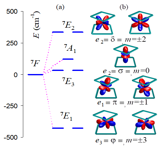
Fig. 6.29. (a) The CASCCF levels corresponding to the LF splitting of the 7F spectral term (with the barycenter conventionally shifted to the origin) (b) the LF one-electron effective scheme based on CASSCF results.
The simple description of the spectral terms from the f8 shell as single configurations, with respect of the placement of the b (or, equivalently, doubly occupied) component, is due to the D4d point group characteristics, that allow the complete symmetry separation inside the set of involved Slater determinants. The LF scheme corresponds to the following ordering of the f orbitals, taken in the axial labelling: {x(x2-3y2), y(3x2-y2)}, {xz2 ,yz2 }, z3, {xyz, z(x2-y2)}. As schematized in Figure 6.29, the highest energy is achieved by the m=+/-2 components, since, having the lobes oriented directly toward the tetragonal frame of the ligand donors, these AOs are experiencing the highest LF perturbation. The least perturbed are the m=+/-3 companions, whose lobes are escaping completely the orientation toward the ligands. Then, is difficult to decide qualitatively the ordering of other two. Apparently, the m=0 escapes from directed metal-ligand overlap, pointing to the rectangular faces of the ligand frame. However, the lone pairs of the nitrogen atoms are intercepting, in non-directed bonding the z3 function which appears higher than the m=+/-1 couple.
In the case of axial symmetry, the extraction of LF parameters is particularly simple:
![]() (6.80)
(6.80)
![]() (6.81)
(6.81)
![]() (6.82)
(6.82)
The equations (6.80)-(6.82) are
obtained combining the 1.31. and 2.10 formulas from Newmans Crystal Field
Handbook (Newman and Ng 2000). The computed LF parameters, ![]() (with k=2, 4,
6), aside with the results of several other numerical experiments, are
presented in Table 6.13. One observes a reasonable agreement between the column
(a) containing the reference of Ishikawa's fit parameters (Ishikawa et al 2003;
Ishikawa et al 2002) and the column (b) with actual computation results, certifying
that the CASSCF states yield a good simulation of the LF phenomenology. Table
6.13 also contains other numeric experiments. In case (c), the e3 < e1 <
b2 < e2 canonical MO energies were used as LF surrogate. In this case the
(with k=2, 4,
6), aside with the results of several other numerical experiments, are
presented in Table 6.13. One observes a reasonable agreement between the column
(a) containing the reference of Ishikawa's fit parameters (Ishikawa et al 2003;
Ishikawa et al 2002) and the column (b) with actual computation results, certifying
that the CASSCF states yield a good simulation of the LF phenomenology. Table
6.13 also contains other numeric experiments. In case (c), the e3 < e1 <
b2 < e2 canonical MO energies were used as LF surrogate. In this case the ![]() amounts
obey, roughly, the expected range, but are not completely satisfactory, in line
with the fact that the canonical MO energies have no immediate physical
meaning.
amounts
obey, roughly, the expected range, but are not completely satisfactory, in line
with the fact that the canonical MO energies have no immediate physical
meaning.
Table 6.13. The Ligand Field parameters for the [Pc2TbIII]- complex, as resulted from: (a) Ishikawa's fit to experiment (Ishikawa et al 2003; Ishikawa et al 2002), (b) states of a CASSCF(8,7) calculation (c) canonical MO energies, (d) crude perturbation of Tb(III) with the Mulliken point charges of the atoms from ligands (e) the electrostatic perturbation with the Effective Fragment Potentials (EFP) method. All quantities are in cm-1.
|
|
(a) |
(b) |
(c) |
(d) |
(e) |
|
|
414 |
440.0 |
388.0 |
44.1 |
312.9 |
|
|
-228 |
-173.7 |
-101.1 |
-47.0 |
-51.3 |
|
|
33 |
37.2 |
34.4 |
2.3 |
2.6 |
In column (d) of Table 6.13 the Tb(III) ion was placed in the electrostatic field generated by point charges taken from the Mulliken populations on the atoms from the two Pc2- ligands. In the (e) case the ligands were replaced by EFPs (Effective Fragment Potentials) (Day et al 1996). The EFP method was initially designed for solvent effects, but we consider it potentially useful to also mimic a LF environment. The EFP of the ligands are constructed as a series of electrostatic terms from, monopole to octupoles, placed at the atomic sites, as well as in the middle of the bonds from the ligand skeleton. The described numeric experiments are illustrating the hierarchy in the amount of electrostatic perturbations contained in the effective LF parameters, from point charge (column d) to multipolar (column e). One observes that, in spite of the ionic nature of the lanthanide complexes, the electrostatic approximation does not work well. However, as phenomenology, with parameters fitted to experiment or advanced calculation methods, it forms the core of fruitful Ligand Field methods.
In the section 6.4.2 it was discussed that second order perturbation (PT2) treatments, applied non-variationaly after the CASSCF step can improve (or not) the results. However, the PT2 is rather superfluous for the lanthanide complexes, as was early probed (Paulovic et al 2004), the costly procedures (as computing time and storage demands) bringing only small changes to the CASSCF results. In general, the PT2 terms are believed to compensate the effects of a limited active space, if orbitals important for the problem at hand are not explicitly identified and picked for the configuration interaction set. In the lanthanide complexes, the active space made of the f-type orbitals, with their corresponding electron occupancy, are reflecting well ligand field phenomenology and related properties in the spectroscopy and magnetism. The MRPT multi-reference second order perturbation method from GAMESS yields the {536.7, -149.4, 40.7} values (in cm-1) for the respective {A2,0r2, A4,0r4, A6,0r6} parameter series. With the Orca program and its NEVPT2 routine, one obtains the {446.6, -147.4, 36.4} set (in cm-1). Both PT2 evaluations remain close to initial CASSCF level, which is reliable in numerical respects and clearer in conceptual sense, revealing itself as the ab initio facet of the Ligand Field theory in the case of lanthanide complexes.
Must also point the appropriateness of the effective core potential basis sets (ECP), like the Stevens- Basch- Krauss- Jasien- Cundari (SBKJC) (Stevens et al 1984; Cundari and Stevens 1993), used here. This is because, having a rather pure f character as final orbitals of the CASSCF iterations, the good representation of the f shell in the basis set is the sufficient condition for the account of the LF regime. The replacement of core electrons by the effective potentials may affect the numeric results of some overall quantities, such as formation energies, but do not impinges upon the account of magnetic and optical properties confined within f-shell causalities. Being relatively cheap, as computation effort, and easing the convergence, the ECP basis sets represent a reasonable choice in the computational account of the f-based compounds.
Table 6.14. The levels resulted from multi-configuration Spin-Orbit (CASSCF-SO) calculation on [Pc2Tb]- complex, dichotomized in the sequences related with the parent J quantum numbers in the free Tb(III).
|
J=6 |
E(cm-1) |
|
J=5 |
E(cm-1) |
|
J=4 |
E(cm-1) |
|
1 |
0.0 |
|
14 |
2190.1 |
|
25 |
3881.2 |
|
2 |
0.0 |
|
15 |
2190.1 |
|
26 |
3881.2 |
|
3 |
307.8 |
|
16 |
2299.7 |
|
27 |
3966.2 |
|
4 |
307.8 |
|
17 |
2299.7 |
|
28 |
3966.2 |
|
5 |
479.8 |
|
18 |
2412.3 |
|
29 |
4041.4 |
|
6 |
479.8 |
|
19 |
2412.3 |
|
30 |
4041.4 |
|
7 |
509.8 |
|
20 |
2443.3 |
|
31 |
4098.4 |
|
8 |
515.1 |
|
21 |
2443.3 |
|
32 |
4098.4 |
|
9 |
515.1 |
|
22 |
2503.4 |
|
33 |
4187.2 |
|
10 |
527.5 |
|
23 |
2503.4 |
|
|
|
|
11 |
527.5 |
|
24 |
2512.1 |
|
|
|
|
12 |
530.5 |
|
|
|
|
|
|
|
13 |
530.5 |
|
|
|
|
|
|
|
J=3 |
E(cm-1) |
|
J=2 |
E(cm-1) |
|
J=1 |
E(cm-1) |
|
34 |
5246.0 |
|
41 |
6064.8 |
|
46 |
6853.1 |
|
35 |
5306.4 |
|
42 |
6394.6 |
|
47 |
7073.2 |
|
36 |
5306.4 |
|
43 |
6394.6 |
|
48 |
7073.2 |
|
37 |
5313.6 |
|
44 |
6404.0 |
|
|
|
|
38 |
5313.6 |
|
45 |
6404.0 |
|
J=0 |
E(cm-1) |
|
39 |
5419.2 |
|
|
|
|
49 |
7335.9 |
|
40 |
5419.2 |
|
|
|
|
|
|
The next step of the calculation represents the adding of the necessary spin-orbit (SO) interaction, which is done taking the CASSCF function as basis, and applying the keywords specific in the used code. The SO treatment is non-variational, the CASSCF-SO results modelling the outcome of a LF-SO interaction.
For the 7F spectral term, there are 49 levels, as result of the combined LF-SO split, grouped in doubly degenerate or singly degenerate sequences, as can be seen in the Table 6.14. The larger gaps are due to the SO coupling, assignable to the J=6 to 0 quantum numbers from the free ion. Each J set is split in its 2J+1 components (including in the count the content of the doublets) by the action of the Ligand Field potential. The Figure 6.30 illustrates, in the left side, the SO in the free Tb3+ ion, to be compared with the full LF-SO diagram from the right side.
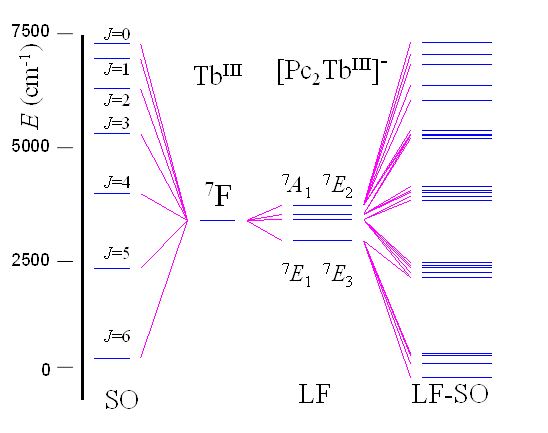
Fig. 6.30. The CASCCF results corresponding to Ligand Field split of the 7F atomic term (in the center of the diagram) and full spectrum from CASSCF-SO (Spin-Orbit) calculations, accounting for the combined LF-SO effects (right side). As comparison: the J levels simulated by CASSCF-SO on Tb(III) free ion (left side). The lowest LF-SO multiplet (lower-right corner) corresponds to the LF split of the J=6 (7F6) atomic SO multiplet.
An advanced handling can be
realized inserting the action of the magnetic field on the CASSCF-SO
Hamiltonian, opening the way for the ab initio account of the magnetic
properties, particularly revealing the anisotropy features. An essential step
is the extraction of ![]() ,
, ![]() ,
, ![]() matrix
elements from the black box of the ab initio SO calculations (Koseki et al
2001; Fedorov et al 2003) which, altogether with the easily available spin
components, allow the construction of the Zeeman matrices for the given
CASSCF-SO problem. Having the field dependence implemented in the full ab
initio Hamiltonian, the magnetization of the i-th level is taken as derivative
of the corresponding eigenvalue with respect of the field:
matrix
elements from the black box of the ab initio SO calculations (Koseki et al
2001; Fedorov et al 2003) which, altogether with the easily available spin
components, allow the construction of the Zeeman matrices for the given
CASSCF-SO problem. Having the field dependence implemented in the full ab
initio Hamiltonian, the magnetization of the i-th level is taken as derivative
of the corresponding eigenvalue with respect of the field: ![]() .Scanning the
response functions
.Scanning the
response functions ![]() of the eigenvalue
"i", with respect to the magnetic field applied at various
orientations, described by the azimuthal q
and polar j coordinate, the modelling
produces objects that can be called state-specific magnetization functions. Represented
in polar diagrams as 3D shapes, these are characterizing the anisotropy of the
given states (see Figures 6.31 and 6.32). In such a polar diagram, for a given q, j
direction, the distance between the origin and the represented surface is equal
to the response,
of the eigenvalue
"i", with respect to the magnetic field applied at various
orientations, described by the azimuthal q
and polar j coordinate, the modelling
produces objects that can be called state-specific magnetization functions. Represented
in polar diagrams as 3D shapes, these are characterizing the anisotropy of the
given states (see Figures 6.31 and 6.32). In such a polar diagram, for a given q, j
direction, the distance between the origin and the represented surface is equal
to the response, ![]() , to the magnetic field
perturbation. In isotropic systems the magnetic response is constant,
irrespective the direction, the map being a sphere. In anisotropic cases, the
response is differentiated, most often revealed in bi-lobate shape, i.e. with a
maximal response along a given axis (named of easy magnetization),
perpendicular to a plane recording null or minimal response (where the radius
of the polar representation, proportional with the response is contracted nearby
the magnetic center).
, to the magnetic field
perturbation. In isotropic systems the magnetic response is constant,
irrespective the direction, the map being a sphere. In anisotropic cases, the
response is differentiated, most often revealed in bi-lobate shape, i.e. with a
maximal response along a given axis (named of easy magnetization),
perpendicular to a plane recording null or minimal response (where the radius
of the polar representation, proportional with the response is contracted nearby
the magnetic center).
The Figure 6.31 shows the
magnetization function of the molecular groundstate (the same for the two
degenerate components). One observes that the magnetic anisotropy occurs along
the fourfold axis of the [Pc2Tb]- unit. In Figure 6.32c the magnetization polar
surfaces of all the states originating from the lowest SO multiplet, 7F6, are
shown in relative comparison, on the same scale (omitting the molecular
skeleton). A non-trivial fact is that all the states show axial anisotropy. The
computed maximal extension of the lobes, {9, 7.5, 6, 0, 1.5, 3, 4.5} mB, can be corroborated with the |gJ Jz|
quantities (in Bohr Magnetons), taken for the ideal gJ=1.5 Lande factor of the
7F6 term and the non-monotonous ordering of the SO states {![]() ,
, ![]() ,
, ![]() ,
,![]() ,
, ![]() ,
, ![]() ,
, ![]() },
labelled with the Jz quantum numbers from the J=6 multiplet.
},
labelled with the Jz quantum numbers from the J=6 multiplet.
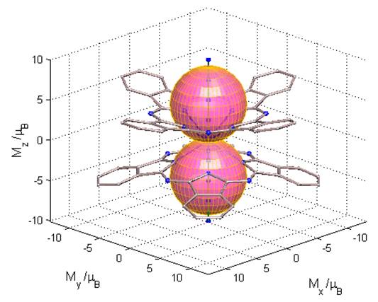
Fig. 6.31. The ab initio computed polar diagram for the magnetization function for the groundstate of the [Pc2Tb]- complex. The 3D frame is in Bohr magneton units, mB. The molecular skeleton is drawn at arbitrary scale.
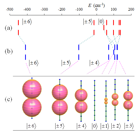
Fig. 6.32. The LF-SO levels corresponding to the 7F6 term: (a) results from Ishikawa's LF-SO parameterization (Ishikawa et al 2003; Ishikawa et al 2002) (b) the CASSCF-SO ab initio calculations (c) the ab initio computed magnetization functions for the considered states. The axes represented trough polar diagrams correspond to the C4 molecular axis. It serves as reference for the size of the lobes, being extended from -10mB to +10mB, with ticks spaced by 2.5mB. The empty bar in the center of panel (c) corresponds to the null magnetization of the state with Jz=0. The magnetization tensors are the same for the degenerate couples with +/-Jz..
The CASSCF-SO computed level
ordering (Figure 6.32b) is slightly different from the LF-SO Ishikawa's
assignment (Figure 6.32a), by the relative placement of the ![]() and
and ![]() components.
However, the comparison of ab initio and fitted results shows a good overall
match, the main features of the spectrum being the same: i) the total gaps are
comparable, with 589 cm-1 from LF-SO fit and 531 cm-1 from ab initio; ii) the
spectral pattern is dominated by the Jz=+/-6 groundstate and the large gap to
the next component Jz=+/-5, all the other states being concentrated in the
upper quarter of the computed or fitted spectra.
components.
However, the comparison of ab initio and fitted results shows a good overall
match, the main features of the spectrum being the same: i) the total gaps are
comparable, with 589 cm-1 from LF-SO fit and 531 cm-1 from ab initio; ii) the
spectral pattern is dominated by the Jz=+/-6 groundstate and the large gap to
the next component Jz=+/-5, all the other states being concentrated in the
upper quarter of the computed or fitted spectra.
Besides, we opine that the
Ishikawa's fit, (Ishikawa et al 2003; Ishikawa et al 2002), in spite of being a
remarkable result, based on an elegant conceptual design, is not completely
unquestionable, with respect to the absolute value of the parameters it provides.
The reason is that, being oriented on the retrieval of magnetic susceptibility
and NMR shifts (experienced by the ligands, due to the central ion), the fit
can offer stable information only about the lowest part of the spectrum, since,
up to the room temperature, the highest levels will not reach significant
thermal population. Therefore, the fit is accurate about the ![]() groundstate and
the occurrence of a large gap to the
groundstate and
the occurrence of a large gap to the ![]() first excited set, but is
less certain about the exact placement of the higher states. Thus, in the
limits of precision of the experiment itself, the match with the computed data
is good.
first excited set, but is
less certain about the exact placement of the higher states. Thus, in the
limits of precision of the experiment itself, the match with the computed data
is good.
At the same time, one may sustain the point that the general goal of the modelling is not just reproducing the nature in matching numbers up to decimal precisions, a semiquantitative performance being satisfactory, if offers meaningful insight, this level being sufficient for interpretation and even for prediction and property design challenges. It seems that, even using moderate complexity for basis sets and taking active spaces related simply with the expected fn phenomenology, the ab initio methods are applicable to LF and magneto-chemical problems of lanthanides. Obeying the facts of chemical intuition and the physics of the weakly interacting systems, the outlined procedure can be proposed as an intuitive and even user-friendly approach.
Hands-on addendum.
In the following we will illustrate calculations details of the above discussed [TbPc2]- complex unit.
Some peoples may think that the CASSCF calculations are overwelming task for computer resources. However, it is perfectly tractable, at a reasonable level of realism. Follow the coming exemplification.
Our strategy is to use owned workstations, dressed each with reasonably high-memory (up to 256 GB, with 12-48 nodes, each).
Being only few users of several workstations, the revenue per user is better than sharing a HPC with tens or hundreds of users. We are about 3-5 users on the owned and cooperation-shared machines, but usually we do not overlap one resources, all being at disposal of one or two users, at a time.
The calculation is most effective if working nodes are grouped in the same machine. So, for CASSCF and subsequent spin-orbit or second-order perturbation it is profitable to have as much memory possible in each machine, than spreading the calculations over many computers.
The [TbPc2]- system is a rather large molecule with 65 the atoms and several hundreds, or few thousands (depending on basis) of orbitals. And yet is piece of cake. The difficulty does not stay in setting the keywords or having bigger machines, but in the wise initialization of input, as above discussed.
We will confine here to a moderate size of basis, since the outcome fits well with the experiment even in these conditions. (see the match to experiment in Table 6.13 and Fig. 6.32)
The body of the input is:
$CONTRL SCFTYP=mcscf�� UNITS=ANGS� !� runtyp=transitn
$CONTRL SCFTYP=mcscf UNITS=ANGS ! runtyp=transitn
�ICHARG=-1 MULT=7 maxit=125 ispher=1
�ECP=READ ! coord=cart
! cityp=aldet
! mplevl=2
�$END
�$SYSTEM Mwords=250 ! memddi=18000
�timlim=90000 $END
�$mcscf cistep=aldet maxit=50
�canonc=.t. ekt=.f. fors=.t. $end
�$det group=C1��
�ncore=166 nels=8 nact=7 nstate=7 sz=3.0�
! ncore=166 nels=8 nact=7 nstate=100 sz=2.0�
�itermx=500 wstate(1)=1,1,1,1,1,1,1
�$end
�$cidet group=C1 clobbr=.t. itermx=500
�ncore=166 nels=8 nact=7 nstate=100 sz=2.0�
�$end
�$trans dirtrf=.t. $end
�$mrmp mrpt=detmrpt $end
�$detpt nptst=7
�iptst(1)=1,2,3,4,5,6,7
�$end
�$TRANST OPERAT=HSO2 ! ZEFF(1)=38
�NFZC=166 NOCC=277 NUMVEC=1 NUMCI=1
�nstate(1)=7
�IROOTS(1)=7
�! JZ=1
�IPRHSO=1 PRTPRM=.t.
�prtcmo=.t.
�$END
�$DRT1 nfzc=166 ndoc=1 nalp=6
�nval=0 fors=.t. group=C1 $END
�$guess guess=moread norb=648 prtmo=.t. $end
�
Some of keywords are active in further steps, after CAS (SO and PT2).
Note that we asked 250 MegaWords per node (Mwords=250), i.e. 2GB for each, i.e. a rather small consume in comparison to the workstation total of about 300GB.
The allocation memory already exceeds the needs per node, as seen in ouput.
NUMBER OF WORDS USED = 186361638
NUMBER OF WORDS AVAILABLE = 250000000
NUMBER OF PASSES = 6
The top comand during the run on six nodes gives:
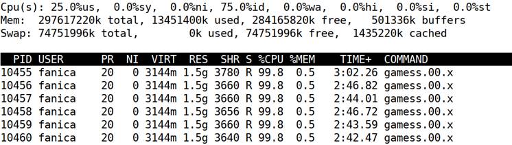
Note in the RES column that the system allocates only 1.5 GB per node i,e, 0.5% of memory.
As mentioned, basis is large, but not the largest. Using, in the present calculation less than 5% of total memory and half of nodes (6 out 12), there is plenty of room to increase much the basis sets or any demanding parameter of the calculation.
As pointed, DFT calculations are not the right procedure for lanthanides. However, if just attempt it, one may see what we should already know, that the memory demands are much smaller in DFT than in CASSCF!
Thus, a bogus DFT consumption is listed as
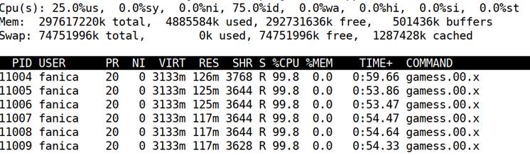
Note that only a meagre demand of about 120MB per node, much smaller than CAS or than the available space (below 0.01%). Emphasize then the cheapness of DFT, in all versions, in all senses.
DFT on lanthanide complexes, in unrestricted frame, can be somehow tamed to convergence, even emulating with specialized control several distinct single-determinant configurations, but this is a physically unsatisfactory surrogate, with severe disorders in the meaning of occupied vs. virtual and alpha vs. beta orbital schemes, incompatible with weak LF paradigm.
For details, consult:
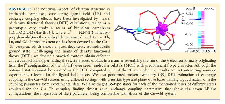
[Ferbinteanu, M; Stroppa, A; Scarrozza, M; Humelnicu, I; Maftei, D; Frecus, B; Cimpoesu, F; On The Density Functional Theory Treatment of Lanthanide Coordination Compounds: A Comparative Study in a Series of Cu-Ln (Ln = Gd, Tb, Lu) Binuclear Complexes, Inorg. Chem. 2017, 56, 16, 9474-9485]